12.4.1 Simple Indices and Time-series Methods
An index used in many climate change detection studies is global mean surface
temperature, either as estimated from the instrumental record of the last 140
years, or from palaeo-reconstructions. Some studies of the characteristics of
the global mean and its relationship to forcing indices are assessed in Section
12.2.3. Here we consider briefly some additional studies that examine the
spatial structure of observed trends or use more sophisticated time-series analysis
techniques to characterise the behaviour of global, hemispheric and zonal mean
temperatures.

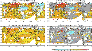
Figure 12.9: (a) Observed surface air temperature trends for 1949
to 1997. (b) Simulated surface air temperature trends for the same period
as estimated from a five-member greenhouse gas plus sulphate ensemble run
with the GFDL R30 model. (c) Observed trends (in colour) that lie outside
the 90% natural variability confidence bounds as estimated from the GFDL
R30 control run. Grey areas show regions where the observed trends are consistent
with the local 49-year temperature trends in the control run. (d) As for
(c) but showing observed 1949 to 1997 trends (in colour) that are significantly
different (as determined with a t-test at the 10% level) from those simulated
by the greenhouse gas plus aerosol simulations performed with the GFDL R30
model (from Knutson et al., 2000). The larger grey areas in (d) than (c)
indicate that the observed trends are consistent with the anthropogenic
forced simulations over larger regions than the control simulations. |
Spatial patterns of trends in surface temperature
An extension of the analysis of global mean temperature is to compare the spatial
structure of observed trends (see Chapter 2, Section
2.2.2.4) with those simulated by models in coupled control simulations.
Knutson et al. (2000) examined observed 1949 to 1997 surface temperature trends
and found that over about half the globe they are significantly larger than
expected from natural low-frequency internal variability as simulated in long
control simulations with the GFDL model (Figure 12.9).
A similar result was obtained by Boer et al. (2000a) using 1900 to 1995 trends.
The level of agreement between observed and simulated trends increases substantially
in both studies when observations are compared with simulations that incorporate
transient greenhouse gases and sulphate aerosol forcing (compare Figure
12.9c with Figure 12.9d, see also Chapter
8, Figure 8.18). While there are areas, such
as the extra-tropical Pacific and North Atlantic Ocean, where the GFDL model
warms significantly more than has been observed, the anthropogenic climate change
simulations do provide a plausible explanation of temperature trends over the
last century over large areas of the globe. Delworth and Knutson (2000) find
that one in five of their anthropogenic climate change simulations showed a
similar evolution of global mean surface temperature over the 20th century to
that observed, with strong warming, particularly in the high latitude North
Atlantic, in the first half of the century. This would suggest that the combination
of anthropogenic forcing and internal variability may be sufficient to account
for the observed early-century warming (as suggested by, e.g., Hegerl et al.,
1996), although other recent studies have suggested that natural forcing may
also have contributed to the early century warming (see Section
12.4.3).
Correlation structures in surface temperature
Another extension is to examine the lagged and cross-correlation structure of
observed and simulated hemispheric mean temperature as in Wigley et al., (1998a).
They find large differences between the observed and model correlation structure
that can be explained by accounting for the combined influences of anthropogenic
and solar forcing and internal variability in the observations. Solar forcing
alone is not found to be a satisfactory explanation for the discrepancy between
the correlation structures of the observed and simulated temperatures. Karoly
and Braganza (2001) also examined the correlation structure of surface air temperature
variations. They used several simple indices, including the land-ocean contrast,
the meridional gradient, and the magnitude of the seasonal cycle, to describe
global climate variations and showed that for natural variations, they contain
information independent of the global mean temperature. They found that the
observed trends in these indices over the last 40 years are unlikely to have
occurred due to natural climate variations and that they are consistent with
model simulations of anthropogenic climate change.
Statistical models of time-series
Further extensions involve the use of statistical models of global,
hemispheric and regional temperature time-series. Note however, that the stochastic
models used in these time-series studies are generally not built from physical
principles and are thus not as strongly constrained by our knowledge of the
physical climate system as climate models. All these studies depend on inferring
the statistical properties of the time-series from an assumed noise model with
parameters estimated from the residuals. As such, the conclusions depend on
the appropriateness or otherwise of the noise model.
Tol and de Vos (1998), using a Bayesian approach, fit a hierarchy of time-series
models to global mean near-surface temperature. They find that there is a robust
statistical relationship between atmospheric CO2 and global mean temperature
and that natural variability is unlikely to be an explanation for the observed
temperature change of the past century. Tol and Vellinga (1998) further conclude
that solar variation is also an unlikely explanation. Zheng and Basher (1999)
use similar time-series models and show that deterministic trends are detectable
over a large part of the globe. Walter et al. (1998), using neural network models,
estimate that the warming during the past century due to greenhouse gas increases
is 0.9 to 1.3°C and that the counter-balancing cooling due to sulphate aerosols
is 0.2 to 0.4°C. Similar results are obtained with a multiple regression
model (Schönwiese et al., 1997). Kaufmann and Stern (1997) examine the
lagged-covariance structure of hemispheric mean temperature and find it consistent
with unequal anthropogenic aerosol forcing in the two hemispheres. Smith et
al. (2001), using similar bivariate time-series models, find that the evidence
for causality becomes weak when the effects of ENSO are taken into account.
Bivariate time-series models of hemispheric mean temperature that account for
boxdiffusion estimates of the response to anthropogenic and solar forcing
are found to fit the observations significantly better than competing statistical
models. All of these studies draw conclusions that are consistent with those
of earlier trend detection studies (as described in the SAR).
In summary, despite various caveats in each individual result, time-series
studies suggest that natural signals and internal variability alone are unlikely
to explain the instrumental record, and that an anthropogenic component is required
to explain changes in the most recent four or five decades.
