12.2.3 Climate Forcings and Responses
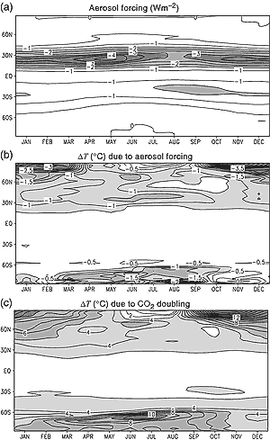
Figure 12.3: Latitude-month plot of radiative forcing and model equilibrium
response for surface temperature. (a) Radiative forcing (Wm-2)
due to increased sulphate aerosol loading at the time of CO2
doubling. (b) Change in temperature due to the increase in aerosol loading.
(c) Change in temperature due to CO2 doubling. Note that the
patterns of radiative forcing and temperature response are quite different
in (a) and (b), but that the patterns of large-scale temperature responses
to different forcings are similar in (b) and (c). The experi-ments used
to compute these fields are described by Reader and Boer (1998). |
The global mean change in radiative forcing (see Chapter
6) since the pre-industrial period may give an indication of the relative
importance of the different external factors influencing climate over the last
century. The temporal and spatial variation of the forcing from different sources
may help to identify the effects of individual factors that have contributed
to recent climate change.
The need for climate models
To detect the response to anthropogenic or natural climate forcing in observations,
we require estimates of the expected space-time pattern of the response. The
influences of natural and anthropogenic forcing on the observed climate can
be separated only if the spatial and temporal variation of each component is
known. These patterns cannot be determined from the observed instrumental record
because variations due to different external forcings are superimposed on each
other and on internal climate variations. Hence climate models are usually used
to estimate the contribution from each factor. The models range from simpler
energy balance models to the most complex coupled atmosphere-ocean general circulation
models that simulate the spatial and temporal variations of many climatic parameters
(Chapter 8).
The models used
Energy balance models (EBMs) simulate the effect of radiative climate forcing
on surface temperature. Climate sensitivity is included as an adjustable parameter.
These models are computationally inexpensive and produce noise-free estimates
of the climate signal. However, EBMs cannot represent dynamical components of
the climate signal, generally cannot simulate variables other than surface temperature,
and may omit some of the important feedback processes that are accounted for
in more complex models. Most detection and attribution approaches therefore
apply signals estimated from coupled Atmosphere Ocean General Circulation Models
(AOGCMs) or atmospheric General Circulation Models (GCMs) coupled to mixed-layer
ocean models. Forced simulations with such models contain both the climate response
to external forcing and superimposed internal climate variability. Estimates
of the climate response computed from model output will necessarily contain
at least some noise from this source, although this can be reduced by the use
of ensemble simulations. Note that different models can produce quite different
patterns of response to a given forcing due to differences in the representation
of feedbacks arising from changes in cloud (in particular), sea ice and land
surface processes.
The relationship between patterns of forcing and response
There are several reasons why one should not expect a simple relationship between
the patterns of radiative forcing and temperature response. First, strong feedbacks
such as those due to water vapour and sea ice tend to reduce the difference
in the temperature response due to different forcings. This is illustrated graphically
by the response to the simplified aerosol forcing used in early studies. The
magnitude of the model response is largest over the Arctic in winter even though
the forcing is small, largely due to ice-albedo feedback. The large-scale patterns
of change and their temporal variations are similar, but of opposite sign, to
that obtained in greenhouse gas experiments (Figure 12.3,
see also Mitchell et al., 1995a). Second, atmospheric circulation tends to smooth
out temperature gradients and reduce the differences in response patterns. Similarly,
the thermal inertia of the climate system tends to reduce the amplitude of short-term
fluctuations in forcing. Third, changes in radiative forcing are more effective
if they act near the surface, where cooling to space is restricted, than at
upper levels, and in high latitudes, where there are stronger positive feedbacks
than at low latitudes (Hansen et al., 1997a).
In practice, the response of a given model to different forcing patterns can
be quite similar (Hegerl et al., 1997; North and Stevens, 1998; Tett et al.,
1999). Similar signal patterns (a condition often referred to as degeneracy)
can be difficult to distinguish from one another. Tett et al. (1999) find substantial
degeneracy between greenhouse gas, sulphate, volcanic and solar patterns they
used in their detection study using HadCM2. On the other hand, the greenhouse
gas and aerosol patterns generated by ECHAM3 LSG (Hegerl et al., 2000) are more
clearly separable, in part because the patterns are more distinct, and in part
because the aerosol response pattern correlates less well with ECHAM3 LSGs
patterns of internal variability. The vertical patterns of temperature change
due to greenhouse gas and stratospheric ozone forcing are less degenerate than
the horizontal patterns.
Summary
Different models may give quite different patterns of response for the same
forcing, but an individual model may give a surprisingly similar response for
different forcings. The first point means that attribution studies may give
different results when using signals generated from different models. The second
point means that it may be more difficult to distinguish between the response
to different factors than one might expect, given the differences in radiative
forcing.