Climate Change 2001: The Scientific Basis

9.3.2.1 Summary

First we note results assessed here that reconfirm results from the SAR:

As the climate warms, Northern Hemisphere snow cover and sea-ice extent decrease. The globally averaged precipitation increases.
As the radiative forcing of the climate system changes, the land warms faster than the ocean. The cooling effect of tropo-spheric aerosols moderates warming both globally and locally.
The surface air temperature increase is smaller in the North Atlantic and circumpolar Southern Ocean regions.
Most tropical areas, particularly over ocean, have increased precipitation, with decreases in most of the sub-tropics, and relatively smaller precipitation increases in high latitudes.
The signal to noise ratio (from the multi-model ensemble) is greater for surface air temperature than for precipitation.

A second category of results assessed here are those that are new since the SAR:

There are many more model projections for a given scenario, and more scenarios. The greater number of model simulations allows us to better quantify patterns of climate change for a given forcing and develop a measure of consistency among the models.
Including the direct effect of sulphate aerosols according to an IS92a type estimate reduces global mean mid-21st century warming. The indirect effect, not included in most AOGCM experiments to date, is acknowledged to be uncertain, as discussed in Chapter 6.
The geographic details of various forcing patterns are less important than differences among the models’ responses for the scenarios considered here. This is the case for the global mean as well as for patterns of climate response. Thus, the choice of model and the choice of scenario are both important.

9.3.3 Range of Temperature Response to SRES Emission Scenarios

This section investigates the range of future global mean temperature changes resulting from the thirty-five final SRES emissions scenarios with complete greenhouse gas emissions (Nakic´enovic´ et al., 2000). This range is compared to the expected range of uncertainty due to the differences in the response of several AOGCMs. Forcing uncertainties are not considered in these calculations. As well as envelope results that incorporate all the SRES scenarios, six specific SRES scenarios are considered. These are the four illustrative marker scenarios A1B, A2, B1 and B2 and two further illustrative scenarios from the A1 family representing different energy technology options; A1FI and A1T (see Section 9.3.1.3 and Box 9.1). For comparison, results are also shown for some of the IS92 scenarios. As discussed in Section 9.3.1.3 some AOGCMs have run experiments with some or all of the four draft marker scenarios. In order to investigate the temperature change implications of the full range of the final SRES scenarios, a simple climate model is used as a tool to simulate the AOGCM results (Wigley and Raper, 1992; Raper et al., 1996, 2001a). The tuning of the simple model to emulate the different AOGCM results is described in Appendix 9.1. The original SRES MiniCAM (Mini Climate Assessment Model from the Pacific Northwest National Laboratory, USA) scenarios did not contain emissions for the reactive gases CO, NMVOCs, and NO_x (Nakic´enovic´ et al., 2000). To facilitate the calculations, the MiniCAM modelling team provided emissions paths for these gases.

For the six illustrative SRES scenarios, anthropogenic emissions are shown for CO₂ in Chapter 3, Figure 3.12, tabulated for CH₄ and N₂O in Appendix II and shown in Nakic´enovic´ et al. (2000), and shown for SO₂ in Chapter 5, Figure 5.13. It is evident that these scenarios encompass a wide range of emissions. Note in particular the much lower future sulphur dioxide emissions for the six SRES scenarios compared with the IS92a scenario.

The calculation of radiative forcing from the SRES emission scenarios for the temperature projections presented here follows closely that described in Chapters 3, 4, 5 and 6, with some exceptions as described below. Further details of the forcing for the collective procedures (MAGICC model) are given by Wigley (2000). Atmospheric concentrations of the greenhouse gases are calculated from the emissions using gas cycle models. For CO₂, the model of Wigley (1993) is used and as described therein, the CO₂ fertilisation factor is adjusted to give a balanced 1980s mean budget. To be consistent with Chapter 3, climate feedbacks are included and the model has been tuned to give results that are similar to those of the Bern-CC and ISAM models for a climate sensitivity of 2.5°C (Chapter 3, Figure 3.12). The strength of the climate feedbacks on the carbon cycle are very uncertain, but models show they are in the direction of greater temperature change giving greater atmospheric CO₂ concentration. The climate feedbacks in the Bern-CC model are greater than those of the ISAM model and the feedback strength used here is about half as big as that in the ISAM model. The gas cycle models for CH₄ and N₂O and the other trace gases are identical to those used in Chapter 4. The concentrations for the main greenhouse gases for the six SRES scenarios are shown in Chapter 4, Figure 4.14.

Except for the treatment of organic carbon (OC), black carbon (BC) and indirect aerosol forcing, the method of calculation for the radiative forcing follows closely that described in Chapter 6 and includes tropospheric ozone, halocarbons, and stratospheric ozone. For OC and BC this report’s best estimate forcing values for the present day given in Chapter 6, Table 6.11 are used. As pointed out in Chapter 5, past and future emissions of OC and BC are uncertain. Here fossil OC and BC direct aerosol forcings are considered together and are scaled linearly with SO₂ emissions. Biomass burning OC and BC aerosol direct forcings are both scaled with gross deforestation. First (cloud albedo) indirect sulphate aerosol forcing components are included and scaled non-linearly with SO₂ emissions as derived by Wigley (1991). A present day indirect sulphate aerosol forcing of –0.8 Wm^-2 is assumed. This is the same value as that employed in the SAR. It is well within the range of values recommended by Chapter 6, and is also consistent with that deduced from model simulations and the observed temperature record (Chapter 12).

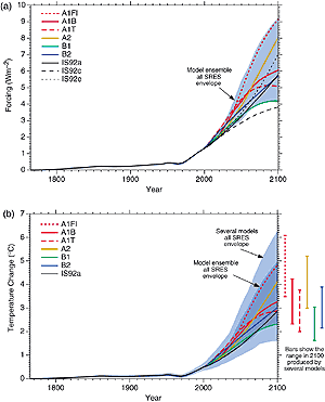
Figure 9.13: Simple model results. (a) Estimated historical anthropogenic radiative forcing followed by radiative forcing for the four illustrative SRES marker scenarios and for two additional scenarios from the A1 family illustrating different energy technology options. The blue shading shows the envelope of forcing that encompasses the full set of thirty-five SRES scenarios. The method of calculation closely follows Chapter 6 except where explained in the text. The values are based on the radiative forcing for a doubling of CO₂ from seven AOGCMs as given in Appendix 9.1, Table 9.A1. The IS92a, IS92c and IS92e forcing is also shown following the same method of calculation. (b) Historical anthropogenic global mean temperature change and future changes for the six illustrative SRES scenarios using a simple climate model tuned to seven AOGCMs. Also for comparison, following the same method, results are shown for IS92a. The dark blue shading represents the envelope of the full set of thirty-five SRES scenarios using the simple model ensemble mean results. The light blue envelope is based on the GFDL_R15_a and DOE PCM parameter settings. The bars show the range of simple model results in 2100 for the seven AOGCM model tunings.

Estimated total historical anthropogenic radiative forcing from 1765 to 1990 followed by forcing resulting from the six illustrative SRES scenarios are both shown in Figure 9.13a. It is evident that the six SRES scenarios considered cover nearly the full range of forcing that results from the full set of SRES scenarios. The latter is shown on figure 9.13a as an envelope since the forcing resulting from individual scenarios cross with time. For comparison, radiative forcing is also shown for the IS92a, IS92c and IS92e scenarios. It is evident that the range in forcing for the new SRES scenarios is wider and higher than in the IS92 scenarios. The range is wider due to more variation in emissions of non-CO₂ greenhouse gases. The shift to higher forcing is mainly due to the reduced future sulphur dioxide emissions of the SRES scenarios compared to the IS92 scenarios. Secondary factors include generally greater tropospheric ozone forcing, the inclusion of climate feedbacks in the carbon cycle and slightly larger cumulative carbon emissions featured in some SRES scenarios.

Figure 9.13b shows the simple climate model simulations representing AOGCM-calibrated global mean temperature change results for the six illustrative SRES scenarios and for the full SRES scenario envelopes. The individual scenario time-series and inner envelope (darker shading) are the average results obtained from simulating the results of seven AOGCMs, denoted “ensemble”. The average of the effective climate sensitivity of these AOGCMs is 2.8°C (see Appendix 9.1). The range of global mean temperature change from 1990 to 2100 given by the six illustrative scenarios for the ensemble is 2.0 to 4.5°C (see Figure 9.14). The range for the six illustrative scenarios encompassing the results calibrated to the DOE PCM and GFDL_R15_a AOGCM parameter settings is 1.4 to 5.6°C. These two AOGCMs have effective climate sensitivities of 1.7 and 4.2°C, respectively (see Table 9.1). The range for these two parameter settings for the full set of SRES scenarios is 1.4 to 5.8°C. Note that this is not the extreme range of possibilities, for two reasons. First, forcing uncertainties have not been considered. Second, some AOGCMs have effective climate sensitivities outside the range considered (see Table 9.1). For example, inclusion of the simple model’s representation of the CCSR/NIES2 AOGCM would increase the high end of the range by several degrees C.

Since the AOGCM SRES results discussed in Section 9.3.1.3 are based on the draft marker SRES scenarios, it is important to note differences that would result from the use of the final SRES scenarios. Based on a comparison using the simple climate model, the final scenarios for the three markers A1B, A2 and B2 give temperature changes that are slightly smaller than those of the draft scenarios (Smith et al., 2001). The main difference is a change in the standardised values for 1990 through 2000, which are common to all these scenarios. This results in higher forcing early in the period. There are further small differences in net forcing, but these decrease until, by 2100, differences in temperature change in the two versions of these scenarios are only 1 to 2%. For the B1 scenario, however, temperature changes are significantly lower in the final version. The difference is almost 20% in 2100, as a result of generally lower emissions across the whole range of greenhouse gases.

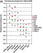
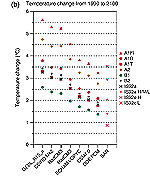
Temperature change results from the simple climate model tuned to individual AOGCMs using the six illustrative SRES scenarios are shown in Figure 9.15. For comparison, analogous results are shown for the IS92a scenario. For direct comparison with the SAR, results are also shown for some of the IS92 scenarios using the SAR forcing and the SAR version of the simple climate model (Kattenberg et al., 1996). The results give rise to conclusions similar to those of Wigley (1999) and Smith et al. (2001), which were drawn from sensitivity studies using the SAR version of the simple climate model. First, note that the range of temperature change for the SRES scenarios is shifted higher than the range for the IS92 scenarios, primarily because of the higher forcing as described above.

A second feature of the illustrative SRES scenarios is that their relative ranking in terms of global mean temperature changes varies with time (Wigley, 1999; Smith et al. 2001). The temperature-change values of the scenarios cross in about mid-century because of links between the emissions of different gases. In particular, for scenarios with higher fossil fuel use, and therefore carbon dioxide emissions (for example A2), sulphur dioxide emissions are also higher. In the near term (to around 2050) the cooling effect of higher sulphur dioxide emissions more than offsets the warming caused by increased emissions of greenhouse gases in scenarios such as A2. The effect of the high sulphur dioxide emissions in the IS92a scenario is similar. It causes IS92a to give rise to a lower 2030 temperature than any of the specific SRES scenarios considered (Figure 9.15a). The opposite effect is seen for scenarios B1 and B2, which have lower fossil fuel emissions, but also lower sulphur dioxide emissions. This leads to a larger near-term warming. In the longer term, however, the level of emissions of long-lived greenhouse gases such as carbon dioxide and nitrous oxide becomes the dominant determinant of the resulting global mean temperature changes. For example, by the latter part of the 21st century, the higher emissions of greenhouse gases in scenario A2 result in larger climate changes than in the other three marker scenarios (A1B, B1 and B2) even though this scenario also has higher sulphur dioxide emissions.

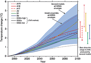
Figure 9.14: As for Figure 9.13b but results are relative to 1990 and shown for 1990 to 2100.

Figure 9.15: Simple model results: Temperature changes from (a) 1990 to 2030 and from (b) 1990 to 2100 for the six illustrative SRES scenarios and IS92a. The bottom axis indicates the AOGCM to which the simple model is tuned. For comparison results are also shown for the SAR version of the simple climate model using SAR forcing with some of the IS92 scenarios (see Kattenberg et al., 1996). IS92a H/M/L refers to the IS92a scenario with climate sensitivity of 1.5, 2.5 and 4.5°C respectively. Also shown are the IS92e scenario with a sensitivity of 4.5°C and the IS92c scenario with a sensitivity of 1.5°C.

Considering the six illustrative scenarios, the bars on the right-hand side of Figure 9.14 show that scenarios A1FI and B1 alone, define the top and bottom of the range of projected temperature changes, respectively. Towards the middle of the range the scenario bars overlap, indicating that most of the projections fall within this region. In the corresponding sea level rise figure, because of the greater intertia in the ocean response, there is a greater overlap in the projected response to the various scenarios (see Chapter 11, Figure 11.12). In addition, the sea level range for a given scenario is broadened by inclusion of uncertainty in land ice estimates.

By 2100, the differences in the surface air temperature response across the group of climate models forced with a given scenario is as large as the range obtained by a single model forced with the different SRES scenarios (Figure 9.15). Given the quasi-linear nature of the simple model, projections which go outside the range as yet explored by AOGCMs must be treated with caution, since non-linear effects may come into play. Further uncertainties arise due to uncertainties in the radiative forcing. The uncertainty in sulphate aerosol forcing is generally characterised in terms of the 1990 radiative forcing. Wigley and Smith (1998) and Smith et al. (2001) examined the effect of this uncertainty on future temperature change by varying the assumed 1990 sulphate radiative forcing by 0.6 Wm^-2 above and below a central value of –1.1 Wm^-2. Reducing the sulphate forcing increased the 1990 to 2100 warming by 0 to 7% (depending on the scenario), while increasing the sulphate forcing decreased warming over the next century by a similar amount. The sensitivity to the uncertainty in sulphate forcing was found to be significantly less in the new scenarios than in the IS92a scenario; in the latter the sensitivity to sulphate forcing was twice as large as the largest value for the SRES marker scenarios. Therefore, the smaller future emissions of sulphur dioxide in the new scenarios significantly lowers the uncertainty in future global mean temperature change due to the uncertain value of present day sulphate aerosol forcing. The climate effects described here use the SRES scenarios as contained in Nakic´enovic´ et al. (2000). Any feedbacks on the socio-economic development path, and hence on emissions, as a result of these climate changes have not been included.

Other reports in this collection