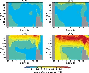
Figure 9.23: Cross-sections of ocean temperature change in the CSIRO Mk2 model stabilisation (3xCO2) experiment (Hirst, 1999).
 Figure 9.23: Cross-sections of ocean temperature change in the CSIRO Mk2 model stabilisation (3xCO2) experiment (Hirst, 1999). |
As mentioned earlier, the basis of the experiments discussed in the SAR is a transient increase of greenhouse gases throughout the integration. In the model integrations presented in this section, the CO2 concentration increases up to a certain value (e.g., a doubling of the CO2 concentration) and then remains constant for the remainder of the integration. Since this type of integration involves integrating the model for very long time periods (at least several centuries) only a few integrations have been performed using AOGCMs. Furthermore, no standard emission scenarios have been used for forcing these model runs and most have used idealised stabilisation values (2xCO2 or 3xCO2 or 4xCO2 for example). Again, in these integrations, the CO2 changes represent the radiative forcing changes of all the greenhouse gases. Results from the models of intermediate complexity are used to help understand the coupled model results, or in some cases, to explore areas where AOGCM integrations do not exist. Experiments where the coupled system is allowed time to reach equilibrium with the radiative forcing clearly show the response times of its various components.
Even after the radiative forcing becomes constant, the surface air temperature continues to increase for many centuries (Figure 9.19) as noted in Section 9.3.4.1. The rate of warming after stabilisation is relatively small (<0.3°C per century, Figure 9.19b); however, the total warming after the radiative forcing stabilises can be significant (more than 1°C) because the warming continues for a long time period (Figure 9.19b). From Figure 9.19, one notes that the rate of warming after stabilisation varies from model to model.
The slow rate of surface air temperature increase occurs as the heat anomaly slowly penetrates to depth in the ocean (Figure 9.23). The rate of penetration is dependent on the models vertical mixing both resolved by the models grid and by the sub-grid scale parametrizations. The effect of the oceanic mixing parametrizations on the coupled model response has been investigated using climate models of intermediate complexity (Figure 9.24): CLIMBER - Ganopolski et al. (2001); Bern 2.5_gm, Bern 2.5_hor - Stocker et al. (1992); Uvic - Fanning and Weaver (1996), Weaver et al. (1998), Wiebe and Weaver (2000); Bern_25, Bern_37 - Siegenthaler and Joos (1992), Joos et al. (1996). The effect on the response of the global mean surface air temperature, thermal expansion (see Chapter 11, Section 11.5.4.1 for a more complete discussion) and THC can be seen by comparing the results obtained from Stockers (Bern 2.5) models and the Uvic models (Weaver and Wiebe, 1999). The sub-grid scale mixing para-metrizations vary in the AOGCMs, accounting for much of the difference in the rate of surface warming (as seen in Figure 9.19b).
The thermohaline circulation (THC) response is more complex than that of the surface air temperature in the stablisation integrations (compare Figure 9.19a with Figure 9.25, for example). Typically the THC weakens as the radiative forcing increases (Section 9.3.4.3). After the radiative forcing stabilises, the THC recovers to its control integration value. The initial weakening is caused by the warming of the mixed layer in the ocean and the increase in the freshwater flux in high latitudes. As the radiative forcing stablises, the tendency for the surface fluxes to weaken the THC is balanced by the changes in the ocean heat and water transports and vertical structure. It is found that the time-scale for this recovery varies from model to model (about a century to multi-centuries). Again it is likely that differences in the oceanic mixing are the cause for the differences in the recovery time.
The time rate of change in the radiative forcing also affects both the weakening and recovery of the THC (Figure 9.25). In the GFDL_R15_a model when the CO2 increased at a rate of 1%/yr to doubling, the THC continued to weaken for 70 years after the point at which the CO2 was held constant at the doubled value (year 70). In a second integration, the CO2 increased at a rate of 0.25%/yr to doubling. In this integration, the THC does not weaken after the doubling point (Manabe and Stouffer, 1994), indicating that the behaviour of the THC response is highly dependent on the rate that the radiative forcing changes (Figure 9.25).
Finally, it is important to note that the transient THC response (i.e., the weakening) is quite different from the equilibrium response of the THC (i.e., little change). This fact makes the interpretation of comparisons between palaeo-proxy data and coupled model results presented here difficult, since one needs to know the details of the changes in the radiative forcing and resolve relatively small time-scales in the proxy record.
|
Other reports in this collection |