8.4 Coupled Climate Models - Some Methodologies
8.4.1 Model Initialisation
 

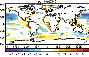
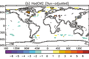
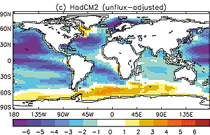
Figure 8.1: Decadal mean SST errors relative to the GISST climatology
for (a) the non-flux adjusted model HadCM3 (Gordon et al., 2000), (b) the
previous generation, flux adjusted model HadCM2 (Johns et al. 1997), (c)
the HadCM2 model when run without flux adjustments (Gregory and Mitchell,
1997). The figures are from representative periods after at least 100 years
of each control run. Multi-century drifts in each run are much smaller than
the differences between the runs. The errors are smallest in (b), because
the flux adjustments were chosen specifically to minimise the errors. The
errors in (c) result from a number of complex feedbacks. The model was designed
to work in flux adjusted mode and it is possible that the non-flux adjusted
SST errors could have been reduced by relatively minor tuning
of the model. |
In this chapter, we assess climate models on the basis
of their ability to simulate present and past climates. What it means to simulate
a particular climate state is linked to the question of model initialisation.
Ideally, given a perfect model, and perfect knowledge
of the present climate state, one could simply initialise a climate model with
the present state. Then, given perpetual present day forcing (from trace substances
and solar radiation), one might expect the model to remain close to the present
state, perhaps with some level of variability. However, in practice, this ideal
is not achieved and a model initialised in this way adjusts from the initial
state. This adjustment has been characterised by two time-scales (Bryan, 1998):
in the initial fast adjustment, the atmosphere, land surface, ocean
mixed layer and sea ice reach a state of near equilibrium, typically taking
5 to 50 years. Surface temperature error patterns (e.g., Figure
8.1a) are generally established on this time-scale, and persist over many
centuries of integration, but there typically remain slight imbalances in the
surface heat and fresh water fluxes. These imbalances drive a second, slower,
adjustment phase (often called climate drift) which takes place
over centuries to millennia and involves adjustment of the deep ocean to the
surface imbalances. This climate drift can make interpretation of
transient climate change simulations difficult, so models are generally allowed
to adjust to a state where such drifts have become acceptably slow, before starting
climate change simulations. A number of techniques have been used to achieve
this (see Stouffer and Dixon, 1998), but it is not possible, in general, to
say which of these procedures gives better initial conditions for
a climate change projection run.
A number of model runs have now been made which are forced by the historical
record of natural and anthropogenic forcing from the mid-19th century to the
present. As well as avoiding the cold start problem in climate projections
(SAR Chapter 6, Section 6.2.4 and Chapter 9), these runs
can be compared against historical observations and form a valuable model evaluation
tool (Section 8.6.1).
8.4.2 Flux Adjustment and Energy Transports
Given present day greenhouse gas concentrations, most coupled models at the
time of the SAR had difficulty in obtaining a stable climate near to the present
day state. Therefore flux adjustment terms were often added to the
surface fluxes of heat, water and (sometimes) momentum which were passed from
the atmosphere to the ocean model. Flux adjustments are non-physical in that
they cannot be related to any physical process in the climate system and do
not a priori conserve heat and water across the atmosphere-ocean interface.
The flux adjustments were specifically chosen to give a stable and realistic
simulation of present surface climate (especially the sea surface temperature
and sea-ice cover), and were often as large as the annual mean model fluxes
themselves. The need to use such adjustments was clearly a source of uncertainty:
the approach inherently disguises sources of systematic error in the models,
and may distort their sensitivity to changed radiative forcing. Models which
did not use flux adjustment produced unrealistic simulations of fundamental
aspects of the climate system such as the strength of the North Atlantic thermohaline
circulation (SAR Chapter 5, Table 5.5).
Recently a number of coupled models have emerged with greatly improved surface
climatologies without using flux adjustments. Figure 8.1a
shows SST errors from one such model, about 100 years after initialisation.
Errors are generally less than 2°C, and the error pattern shown is stable
over several centuries of integration. However some larger errors are seen,
in particular a cooling in the North Pacific, a warming in the eastern tropical
ocean basins (probably due to a lack of stratocumulus cloud there), and a warming
in the southern ocean. These errors appear to be common to a number of more
recent non-flux adjusted models (Action de Recherche Petite Echelle Grand Echelle/Océan
Parallélisé (ARPEGE/OPA1), Guilyardi and Madec 1997; Climate System
Model (CSM 1.0), Boville and Gent 1998; Hadley Centre Coupled Model (HadCM3),
Gordon et al., 2000), but other models show different error patterns (ARPEGE/OPA2,
Institut Pierre Simon Laplace/Coupled Atmosphere-Ocean-Vegetation Model (IPSL-CM2),
Barthelet et al., 1998a,b). The surface climatologies in several non-flux adjusted
models are now considered good enough and stable enough to use those models
for climate change projections. Typical flux adjusted models do show smaller
SST errors, because the flux adjustments are chosen specifically to minimise
those errors (Figure 8.1b). For comparison, Figure
8.1c shows the SST errors when the older, flux adjusted model was run in
non-flux adjusted mode.
It appears that the success of the recent models which do not require heat
flux adjustments is related to an improved ability to simulate the large-scale
heat balances described in Chapter 7 (Weaver and Hughes,
1996; Guilyardi and Madec, 1997; Johns et al., 1997; Bryan, 1998; Gordon et
al., 2000). Improvements to both atmospheric (Section 8.5.1.2.2)
and oceanic (Section 8.5.2.2) components of the models
have played a part in this advance. Such models have the advantage over flux-adjusted
models that, provided the large-scale balances are obtained using a physically
justifiable choice of model parameters, these models are physically self-consistent
representations of the climate system. However, in some cases only very loose
physical constraints can be placed on the model parameters.
The fresh water budget is more complex than the heat budget because of the
effects of land surface processes, rivers and sea ice. Water budget errors are
potentially far reaching because there is no direct feedback between surface
salinity errors and the surface fresh water flux, for example, persistent freshening
at high latitudes could lead to a collapse of the ocean thermohaline circulation
(Manabe and Stouffer, 1997; see also Chapter 7, Section
7.6.2). Some aspects of the large-scale hydrological cycle are subject to
large observational uncertainty (Wijffels et al., 1992), and this has inhibited
evaluation and improvements in the water budget. Nonetheless, some models are
now able to produce stable multi-century runs without water flux adjustments.
8.4.2.1 Does the use of flux adjustments in a model have
a significant impact on climate change projections?
Marotzke and Stone (1995) show that using flux adjustment to correct surface
errors in the control climate does not necessarily correct errors in processes
which control the climate change response. Flux adjustments can also result
in spurious multiple equilibrium states of the tropical (Neelin and Dijkstra,
1995) and thermohaline (Dijkstra and Neelin, 1999) ocean circulation. On the
other hand, a good representation of, say, sea-ice extent may be important to
produce the correct magnitude of ice-albedo feedback under climate change, and
it may be preferable to use flux adjustments to give a good sea-ice distribution
than to omit the flux adjustments but to have a poorer sea-ice extent. Overall,
differences have been seen in the climate change response of flux adjusted and
equivalent non-flux adjusted models (Fanning and Weaver, 1997b; Gregory and
Mitchell, 1997), but it is not clear whether the differences are due to the
flux adjustment itself, or to the systematic errors in the non-flux adjusted
model. The only practical way to resolve this issue may be to continue the progress
which has been made towards models which achieve good surface climatology without
flux adjustment, whereupon the effect of flux adjustments will cease to be of
concern.
